Tensor Train Optimization Tutorial
This library includes extensible functionality for directly optimizing tensor trains.
Suppose we want to optimize a tensor train tt to minimize some function f(tt). Using automatic differentiation, we would be able to automatically compute the gradients of this function in all of the entries of tt. This is however not a good idea; there are many symmetries in the tensor train format and this approach works very badly in practice.
Instead we optimize tensor trains using Riemannian (conjugate) gradient descent. It turns out that Riemannian gradients for tensor trains can be computed relatively efficiently, and they provide faster and more numerically stable convergence.
Tensor completion
Specifically for the problem of solving the tensor completion problem we have implemented the TensorTrainLineSearch class. Below we see it in action:
[1]:
from ttml.tensor_train import TensorTrain
from ttml.tt_rlinesearch import TensorTrainLineSearch
import matplotlib.pyplot as plt
import numpy as np

# Create a dummy problem
dims = (5, 4, 5, 10)
N = 1000
# Randomly choose indices
idx = np.stack([np.random.choice(d, size=N) for d in dims], axis=1)
y = np.exp(np.sum(idx, axis=1) / 10)  # Function is exp sum

# Initialize random tensor train with rank 2
tt = TensorTrain.random(dims, 2)

# Initialize an optimizer for the tensor train completion problem
optim = TensorTrainLineSearch(tt, y, idx, task="regression")


# Do 50 steps of optimization
losses = []
grads = []
stepsizes = []
for i in range(50):
    loss, grad, stepsize = optim.step()
    losses.append(loss)
    grads.append(-grad)
    stepsizes.append(stepsize)

# Plot the results
plt.figure(figsize=(14, 4))
plt.subplot(1, 3, 1)
plt.title("Loss")
plt.yscale("log")
plt.plot(losses)
plt.subplot(1, 3, 2)
plt.title("Gradients")
plt.plot(grads)
plt.yscale("log")
plt.subplot(1, 3, 3)
plt.title("Stepsize")
plt.plot(stepsizes)
plt.show()
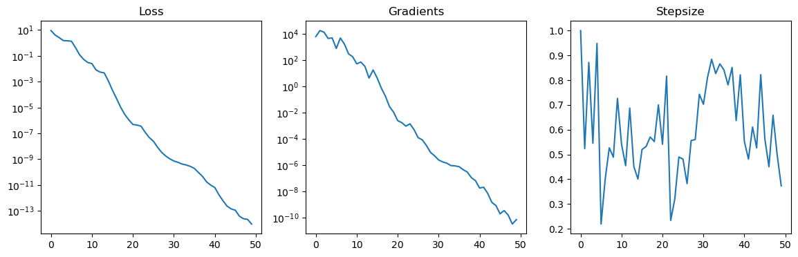
We see that the loss is quickly and linearly convergening to 0. This is because the underlying function can be exactly represented by a rank 2 tensor train.
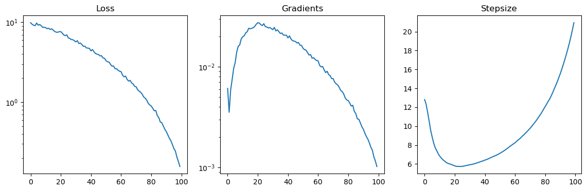
This optimization problem minimizes a mean squared error. For classification problems we may want to minimize cross entropy loss instead. This can be done by supplying the task="classification" keyword argument. Below we solve a simple classification problem, but in this case convergence is even faster so we only do 10 steps.
[2]:
# Reuse previous y to create ballanced classification problem
y_classification = (y > np.median(y)).astype(int)

# Initialize random tensor train with rank 2
tt = TensorTrain.random(dims, 2)

# Initialize an optimizer for the tensor train completion problem
optim = TensorTrainLineSearch(tt, y, idx, task="classification")


# Do 10 steps of optimization
losses = []
grads = []
stepsizes = []
for i in range(10):
    loss, grad, stepsize = optim.step()
    losses.append(loss)
    grads.append(-grad)
    stepsizes.append(stepsize)

# Plot the results
plt.figure(figsize=(14, 4))
plt.subplot(1, 3, 1)
plt.title("Loss")
# plt.yscale("log")
plt.plot(losses)
plt.subplot(1, 3, 2)
plt.title("Gradients")
plt.plot(grads)
plt.yscale("log")
plt.subplot(1, 3, 3)
plt.title("Stepsize")
plt.plot(stepsizes)
plt.show()

Parameters for TensorTrainLineSearch
There are many options for TensorTrainLineSearch. We highlight the most important ones.
sample_weightsWe can associate a positive weight for each sample. This affects both the loss and the gradient, and is useful for example for unbalanced datasets.cg_methodAbove we have used Fletcher-Reeves conjugate gradient descent (cg_method='fr'). We can also use steepest descent (cg_method='sd'), which is slightly faster per step but in general has slower convergence. For Fletcher-Reeves we need to compute the parallel transport of the search direction at each step, which is not necessary for steepest descent.line_search_methodTo determine the stepsize, we use the Armijo conidition by default (line_search_method='armijo'). However we can use the (strong) Wolfe condition instead by usingline_search_method='wolfe'.memoryIfmemory > 1, then we use nonmonotone line search. This means we only require the loss to decrease everymemorysteps.max_stepsizeLimit the maximum stepsize. This can help sometimes with overfitting, but requires specific tuning for each problem. By default the stepsize is unbounded.initial_stepsize_methodThe Armijo and Wolfe line searches both require an initial stepsize. In principle we want that the initial step size satisfies the Armijo/Wolfe conditions, to limit the number of function evaluations required. However, we also want the stepsize to be as large as possible to speed up convergence. All in all this means that the initial step size can have a significant impact on convergence speed.By default we choose the type-1 Barzilai-Borwein stepsize (
'bb1'), but we also support the type-2 BB stepsize ('bb2'). Furthemore we have the Quasi-optimal stepsize based on a linearization of the loss function, as proposed by Steinlechner ('qopt'). Finally with'scalar'we the take twice the difference between current and previous loss value, divided by the derivative of the line search function.auto_scaleIf the optimial stepsize is very large, it can take the optimizer quite a few steps to start using good stepsizes. To avoid this situation, we can setauto_scale=True, which uses the norm of the gradient to better estimate on what scale we should choose the stepsize. This only affects the first step size. This is sometimes necessary for optimizing cross entropy loss.
Stochastic gradient descent
The computation time for each step of gradient descent roughly scales linearly with the number of data points. Therefore if we have a very large number of data points, it makes sense to use stochastic gradient descent to speed things up. In theory stochastic gradient descent can also act as a regularizer. For this purpose we have implemented the Riemannian ADAM stochastic gradient descent algorithm.
Below we consider the same dummy problem as before, but now with many more datapoints. We do stochastic gradient descent with a batch size of 1000, for one epoch of training. Note that batch size can be chosen relatively large, easily up to 10 000. If the batch size is much smaller, then the computation time is dominated by orthogonalization of the tensor trains each step.
[3]:
from ttml.tt_radam import TensorTrainSGD

# Create a dummy problem
dims = (5, 4, 5, 10)
N = 100000
# Randomly choose indices
idx = np.stack([np.random.choice(d, size=N) for d in dims], axis=1)
y = np.exp(np.sum(idx, axis=1) / 10)  # Function is exp sum

# Initialize random tensor train with rank 3
tt = TensorTrain.random(dims, 3)

# Initialize an optimizer for the tensor train completion problem
optim = TensorTrainSGD(tt, y, idx, batch_size=1000, task="regression")

losses = []
grads = []
stepsizes = []
for i in range(100):
    loss, grad, stepsize = optim.step()
    losses.append(loss)
    grads.append(-grad)
    stepsizes.append(stepsize)

# Plot the results
plt.figure(figsize=(14, 4))
plt.subplot(1, 3, 1)
plt.title("Loss")
plt.yscale("log")
plt.plot(losses)
plt.subplot(1, 3, 2)
plt.title("Gradients")
plt.plot(grads)
plt.yscale("log")
plt.subplot(1, 3, 3)
plt.title("Stepsize")
plt.plot(stepsizes)
plt.show()
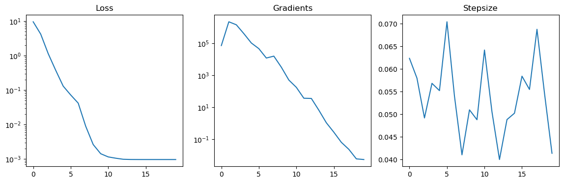
Extending with new loss functions
By default we can only use mean squared error loss and cross entropy loss for the tensor completion problem. We can easily extend the optimizer to use new loss functions. As an example we will show how to implement mean squared error loss with an L2 regularizer.
To do this we need to define two functions: my_loss(tt, y, idx, **kwargs) and my_egrad(tt, y, idx, **kwargs). Here my_loss should return the error we try to minimize, and my_egrad should return the Euclidean gradient of the function. By the Euclidean gradient we mean the sparse gradient of my_loss seen as a function of the dense tensor represented by tt. There will be one gradient value for each index stored in idx.
A simple implementation of these two functions is given below. Note that my_egrad should both return the Euclidean gradient and the loss value.
[4]:
def my_loss(tt, y, idx, **kwargs):
    prediction = tt.gather(idx)
    loss_mse = np.sum((prediction - y) ** 2)
    loss_l2 = np.linalg.norm(prediction) ** 2
    loss = loss_mse + 1e-4 * loss_l2
    return loss


def my_egrad(tt, y, idx, **kwargs):
    prediction = tt.gather(idx)

    loss_mse = np.sum((prediction - y) ** 2)
    loss_l2 = np.linalg.norm(prediction) ** 2
    loss = loss_mse + 1e-4 * loss_l2

    egrad_mse = 2 * (prediction - y)
    egrad_l2 = 2 * np.abs(prediction)
    egrad = egrad_mse + 1e-4 * egrad_l2
    return loss, egrad
Now to use this in TensorTrainLineSearch or TensorTrainSGD we need to tell the meta tensor train optimization class, TensorTrainOptimizer where to look. We do this by adding these functions to the dictionaries tt_opt._loss_func_dict and tt_opt._egrad_func_dict. After that we can use it simply by setting the task= keyword argument to the appropriate value.
[5]:
from ttml import tt_opt

# Register the new loss and egrad
tt_opt._loss_func_dict["my_task"] = my_loss
tt_opt._egrad_func_dict["my_task"] = my_egrad

# Create a dummy problem
dims = (5, 4, 5, 10)
N = 10000
idx = np.stack([np.random.choice(d, size=N) for d in dims], axis=1)
y = np.exp(np.sum(idx, axis=1) / 10)

# Initialize random tensor train with rank 3
tt = TensorTrain.random(dims, 3)

optim = TensorTrainLineSearch(tt, y, idx, task="my_task")

losses = []
grads = []
stepsizes = []
for i in range(20):
    loss, grad, stepsize = optim.step()
    losses.append(loss)
    grads.append(-grad)
    stepsizes.append(stepsize)

# Plot the results
plt.figure(figsize=(14, 4))
plt.subplot(1, 3, 1)
plt.title("Loss")
plt.yscale("log")
plt.plot(losses)
plt.subplot(1, 3, 2)
plt.title("Gradients")
plt.plot(grads)
plt.yscale("log")
plt.subplot(1, 3, 3)
plt.title("Stepsize")
plt.plot(stepsizes)
plt.show()
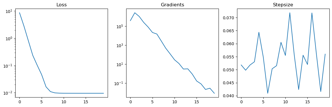
This is the basic functionality, but there three small things we might want to do to improve functionality.
len(y). During optimization it is in general better to use the unormalized version, but for reporting the loss to the user the normalized version makes more sense. The optimizer uses the appropriate version automatically by supplying the normalize keyword to my_loss and my_egrad.sample_weight keyword. In this case we need to be slightly careful, since the sample weights affect loss_mse and egrad_mse, but not loss_l2 and egrad_l2.1e-4. Of course we want the user to specify this coupling constant at runtime. To do this we can add any keyword argument we like to my_loss and my_egrad. This argument can then be specified by the user by adding it to task_kwargs when initializing the optimizer.Let’s take all this into account and upgrade my_loss and my_egrad.
[6]:
def my_loss(tt, y, idx, sample_weight, normalize, my_kwarg=1e-4, **kwargs):
    if sample_weight is None:
        sample_weight = 1.0

    prediction = tt.gather(idx)
    loss_mse = np.sum(((prediction - y) * sample_weight) ** 2)
    loss_l2 = np.linalg.norm(prediction) ** 2
    loss = loss_mse + my_kwarg * loss_l2

    if normalize:
        loss /= len(y)
    return loss


def my_egrad(tt, y, idx, sample_weight, normalize, my_kwarg=1e-4, **kwargs):
    if sample_weight is None:
        sample_weight = 1.0

    prediction = tt.gather(idx)
    loss_mse = np.sum(((prediction - y) * sample_weight) ** 2)
    loss_l2 = np.linalg.norm(prediction) ** 2
    loss = loss_mse + my_kwarg * loss_l2

    egrad_mse = 2 * (prediction - y) * sample_weight
    egrad_l2 = 2 * np.abs(prediction)
    egrad = egrad_mse + my_kwarg * egrad_l2

    if normalize:
        loss /= len(y)
        egrad /= len(y)
    return loss, egrad


tt_opt._loss_func_dict["my_task"] = my_loss
tt_opt._egrad_func_dict["my_task"] = my_egrad
And finally let’s test this function out:
[7]:
# Create a dummy problem
dims = (5, 4, 5, 10)
N = 10000
idx = np.stack([np.random.choice(d, size=N) for d in dims], axis=1)
y = np.exp(np.sum(idx, axis=1) / 10)

# Initialize random tensor train with rank 3
tt = TensorTrain.random(dims, 3)

optim = TensorTrainLineSearch(
    tt, y, idx, task="my_task", task_kwargs={"my_kwarg": 1e-3}
)

losses = []
grads = []
stepsizes = []
for i in range(20):
    loss, grad, stepsize = optim.step()
    losses.append(loss)
    grads.append(-grad)
    stepsizes.append(stepsize)

# Plot the results
plt.figure(figsize=(14, 4))
plt.subplot(1, 3, 1)
plt.title("Loss")
plt.yscale("log")
plt.plot(losses)
plt.subplot(1, 3, 2)
plt.title("Gradients")
plt.plot(grads)
plt.yscale("log")
plt.subplot(1, 3, 3)
plt.title("Stepsize")
plt.plot(stepsizes)
plt.show()
Verifying gradients are correct
After writing our new loss function, we want to verify the gradients are computed correctly. A very useful tool for this is to plot the line search function. At each point along the line search we can also compute the derivatives, and check that the Riemannian derivatives are the same as derivatives obtained through finite difference methods. For these debugging purposes we can use TensorTrainLineSearch.plot_linesearch(). Let’s do this for the loss/egrad functions we wrote above.
It is very easy to make mistakes when defining the gradient egrad function, so we strongly recommend to always do this!
[8]:
tt = TensorTrain.random(dims, 3)

optim = TensorTrainLineSearch(
    tt, y, idx, task="my_task", task_kwargs={"my_kwarg": 1e-3}
)

stepsizes, losses, gradients = optim.plot_linesearch(plot_points=100)
[9]:
plt.figure(figsize=(12,4))
plt.subplot(1,2,1)
plt.title("Line search losses")
plt.plot(stepsizes, losses)

plt.subplot(1,2,2)
plt.title("Line search gradients")
plt.plot(stepsizes, gradients, label="Computed gradients")

# compute finite differences gradients
diffs = np.diff(losses)/np.diff(stepsizes)
diff_stepsizes = 0.5*stepsizes[:-1]+0.5*stepsizes[1:]
plt.plot(diff_stepsizes, diffs, label="Finite differences")
plt.legend()
plt.show()
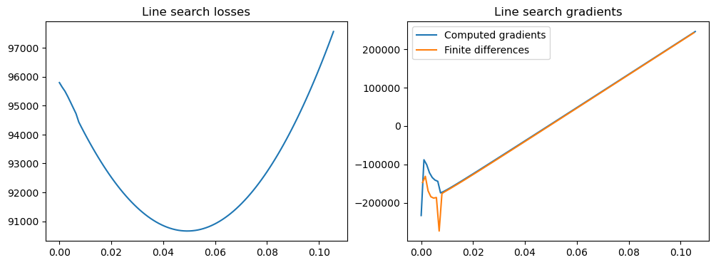
We see that the gradients computed by the line search optimizer and the ones computed using finite differences correspond relatively well (except for a strange peak, probably due to numerical errors). Note that it is normal that they are not precisely the same; this is due to numerical errors on the one hand. For larger step sizes we often see a more significant divergence. This is because we use a retraction instead of a geodesic flow. These two tend to differ more for larger step sizes/gradient norms, and in regions where the manifold is more highly curved.